Concentration Inequalities

Concentration inequalities are used to bound the deviation of a random variable from some number, and they show up everywhere. The treatment here closely follows Chapter 2 of the excellent book High Dimensional Probability, by Vershynin. I have added some intuition, solved exercises, and included some simulations that I felt to be enlightening.

The motivating question will be the following: Consider a coin flipped $N$ times. What is the probability of observing $\frac{3}{4}N$ heads? We will find that the probability decreases exponentially with $N$.

Central Limit Theorem

First, let’s discuss what the central limit theorem (CLT) says about our coin-flipping experiment. Denote the outcome of the $i$th coinflip as the Bernoulli random variable $X_i$ which takes the value 1 if the outcome is heads and 0 if it is tails. Denote the number of heads in an experiment with $N$ tosses as $S_N = \sum_i X_i$. The CLT (in this case, the de Moivre-Laplace theorem) states

$$Z_N \xrightarrow[D]{} N(0,1),$$

where $Z_N = \frac{S_N - Np}{\sqrt{Np(1-p)}}$ is simply the number of heads centered and rescaled. That is, the distribution of the number of heads in our experiment will approach a normal distribution as the number of coin tosses $N$ goes to infinity.

Let’s check it out in R:

ns = c(10,20,50,1000) #Number of coin flips 
p <- 0.5; # It's a fair coin
test_size <- 10000; #Number of times we will simulate the experiment.
toplots <- data.frame();
for (ni in 1:length(ns)){
  n <- ns[ni]
  S_N <- rbinom(n=test_size,size=n,prob=p); # Simulating the experiment by drawing from a binomial distribution
  Z_N <- (S_N-n*p)/sqrt(p*(1-p)*n)
  Z <- rnorm(test_size)
  toplot <- data.frame(x= c(Z_N,Z),
                       group=c(rep("# of Heads",test_size),rep("Normal Distribution",test_size)), 
                       N=rep(n,test_size))
  toplots <- rbind(toplots,toplot)
}
ggplot() + geom_density(data=toplots, aes(x=x,color=group)) +facet_wrap(~N,scales="free")+theme(legend.title  = element_blank(), panel.background = element_blank(), legend.position = "bottom") + xlab("")

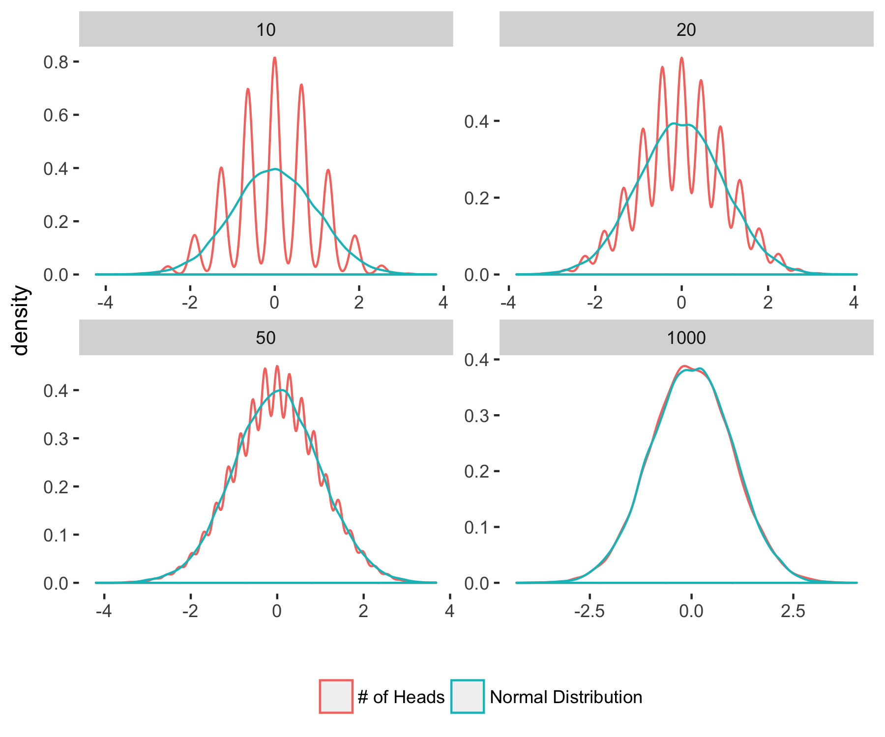
Clearly, the density of $Z_N$ is approaching that of a normal distribution. Can this help us in getting an exponential bound for the probability of the number of heads exceeding $\frac{3N}{4}$? After all, the tails of a Gaussian decay exponentially, so if our random variable of interest approaches a Gaussian, shouldn’t that be enough?

Interestingly, it turns out, this does not work at all! The problem is that the rate at which the $Z_N$ converges in distribution is not nearly fast enough. A quantitative version of the central limit theorem, the Berry-Esseen CLT, says that

$$\big| \mathrm P \left\{ Z_N \geq t \right\} - \mathrm P \left\{ g \geq t \right\} \big| \leq \frac{C}{\sqrt{N} }$$

where $Z \sim N(0,1)$ and $C$ is a constant that we won’t worry about here. The convergence is of order $1/\sqrt{N}$, so it can’t be used to obtain exponential decay. Furthermore, this estimate is sharp. Let’s see for ourselves in some simulated data

p=.5
ns = c(seq(from=10,to=1000, by=10))
empirical_diff <- rep(-1,length(ns)) 
test_size = 1000;
for (ni in 1:length(ns) ){
  n <- ns[ni]
  
  # We want to estimate P{Z_N > t}, and we know that S_N ~ binom(n,p). To use
  # the CDF of S_N, we need to rescale t P{Z_N > t} = P{ S_N > t(\sqrt(p(1-p)N))+ Np}
  ts <- seq(from=-3,to=3,by = 0.1) 
  ts_ <- ts*(sqrt(p*(1-p)*n))+n*p 
  Z_N_gt_t = 1-pbinom(ts_,size = n,prob=p) 
  g_gt_t = 1-pnorm(ts)
  empirical_diff[ni] <- max(abs(Z_N_gt_t - g_gt_t)); # LHS of our inequality
}

berry_esseen <- predict(lm(empirical_diff ~ I(ns^-0.5))) # Let's fit a curve 1/sqrt(N) to compare
toplot <- data.frame(ns=c(ns,ns), probability= c(empirical_diff,berry_esseen),
                     group=c(rep("Empirical Difference",length(ns)),rep("Berry Esseen Bound",length(ns))))
ggplot(toplot, aes(x=ns, probability, color=group)) +geom_line(aes(linetype=group),size=2)+theme(legend.title  = element_blank(), legend.position = "bottom") + xlab("")

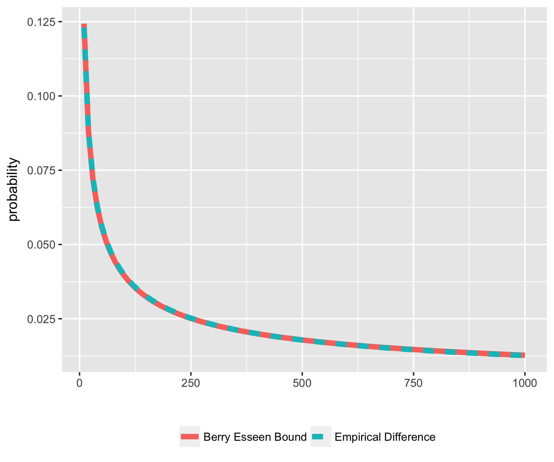
The LHS of our inequality (in blue) decays exactly as $\sim\frac{1}{\sqrt{N}}$. This is really slow, much slower than exponential. So this is why we need concentration inequalities: CLT is not going to help us here.

Concentration Inequalities

In these notes, the bounds we will consider will increase in strength as they increase in the amount of information (i.e. assumptions) about the random variables (or sums of random variables) they are bounding. We begin with Markov Inequality, which uses only non-negativity of the random variable. Then we use it to prove Chebyshev, which uses the variance. By assuming independence, we obtain an exponential bound using Hoeffding. And finally, by taking into account the mean of our random variables, we obtain Chernoff.

Markov & Chebyshev

To get us warmed up, let’s start with the Markov inequality:

For any non-negative random variable $X$, $$\begin{align} \mathrm{P} \{ X \geq t \} \leq \frac{\mathrm {E} X}{t}\end{align}$$

Proof.

Let $(\Omega, \Sigma, \mathrm P)$ be a probability space. $$\begin{align} \mathop{\mathrm E} X &= \int X \, d\mathrm P \\ &\geq \int_{\{ X \geq t\}} X \, d\mathrm P\\ &\geq t \int_{\{ X \geq t\}} \, d\mathrm P \\ &\geq t \cdot \mathrm P \{ X \geq t \} \end{align}$$

This is often a very weak bound, as it does not use anything we know about the random variable $X$. But, it is used in the proof of every other bound in these notes, such as Chebyshev inequality, which uses the variance of $X$ to obtain a concentration bound.

For any random variable $X$, $$\begin{align} \mathrm{P} \{ | X - \mathop{\mathrm E} X| \geq t \} \leq \frac{\mathrm {Var} (X)}{t^2}\end{align}$$

Proof.

We obtain Chebyshev inequality squaring both sides of $|X - \mathop{\mathrm E} X| \geq t$ and applying the Markov inequality. $$\begin{align} \mathrm P \{ | X - \mathop{\mathrm E} X|^2 \geq t^2 \} &\leq \frac{\mathop{\mathrm E} {\left| X - \mathop{\mathrm E} X \right| ^2}}{t^2} \\ &= \frac{\mathrm {Var}(X)}{ t^2} \end{align}$$

Hoeffding’s Inequality

Hoeffding is going to give us the exponential bound for the deviation $\sum_i X_i$ that we are looking for. To do so, it makes a crucial assumption: independence.

To start off, we will prove a special case, where there variables $X_1,…,X_N$ are symmetric Bernoulli. This means that they take the values 1 or -1 with equal probability.

If $X_1,...,X_N$ are symmetric Bernoulli random variables, and $a \in \mathrm R^N$, then for any $t \geq 0$, we have $$\mathrm{P} \left\{\sum_{i=1}^N a_i X_i \geq t \right\} \leq \exp\left( - \frac{t^2}{2 \|a\|^2}\right)$$

Proof.

$$\begin{align*} \mathrm{P} \left\{\sum_{i=1}^N a_i X_i \geq t \right\} & = \mathrm{P} \left\{\exp \left( \lambda \sum_{i=1}^N a_i X_i \right)\geq e^{\lambda t} \right\} \\ & \leq e^{-\lambda t}\mathrm{E} \left\{\exp \left( \lambda \sum_{i=1}^N a_i X_i \right) \right\} \end{align*}$$ where Markov's inequality was used in the second step. Now, by independence: $$\begin{align*} \mathrm{E} \left\{\exp \left( \lambda \sum_{i=1}^N a_i X_i \right) \right\} &= \mathrm{E} \left\{\prod_{i=1}^N \exp(\lambda a_i X_i)\right\}\\ &= \prod_{i=1}^N \mathrm{E} \left\{\exp(\lambda a_i X_i)\right\}. \end{align*}$$ And noting that $X_i$ takes -1 and 1 with probability $1/2$, we can easily compute its expectation as $$\mathrm{E} \left\{\exp(\lambda a_i X_i)\right\} = \frac{e^{\lambda a_i} + e^{-\lambda a_i}}{2} \leq e^{\lambda^2 a_i^2/2}.$$ Because the Taylor series of the exponential, $$e^x = \sum_{k=0}^\infty \frac{x^k}{k!}\\ \frac{e^x + e^{-x}}{2} = \sum_{k=0}^\infty \frac{x^{2k}}{(2k)!}\\ e^{x^2/2} = \sum_{k=0}^\infty \frac{x^{2k}}{2^k (k!)}$$ Therefore, $\frac{e^x + e^{-x}}{2} \leq e^{x^2/2}$. Now, we can plug into the product above, and assuming $\|a\|^2 = 1$: $$\begin{align*} \mathrm{P} \left\{\sum_{i=1}^N a_i X_i \geq t \right\} &\leq e^{-\lambda t}\left( \prod_{i=1}^Ne^{\lambda^2 a_i^2/2}\right) \\ &\leq e^{-\lambda t}\left( e^{\lambda^2 \sum_{i=1}^Na_i^2/2}\right) \\ &= e^{-\lambda t}\left( e^{\lambda^2 /2}\right) \\ &= e^{\lambda^2 /2 - \lambda t } \\ \end{align*}$$ This holds for any $\lambda$, and it is minimized by $\lambda = t$, so we obtain $$\mathrm{P} \left\{\sum_{i=1}^N a_i X_i \geq t \right\} \leq e^{-t^2/2}$$ Of course, by homogeneity, we have it for any $a$ First, note that we can assume $\|a\| = 1$, because $$\mathrm{P} \left\{\sum_{i=1}^N \frac{a_i}{\|a\|} X_i \geq \frac{t}{\|a\|} \right\} \leq e^{-\frac{t^2}{2\|a\|^2}}$$

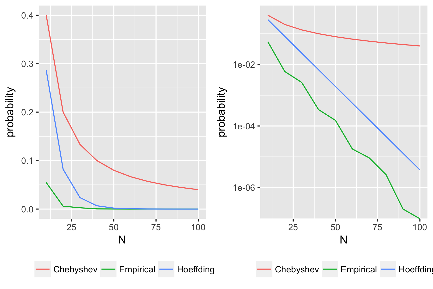
With this theorem in hand, we can obtain bounds for our coin flipping problem. Let $Y_i = 2(X_i-\frac{1}{2})$, which is a symmetric binomial variable.

$$\begin{align*} \mathrm P \{ \sum_i X_i > t \} &= \mathrm P \left\{ \sum_i \left(\frac{Y_i}{2} + \frac{1}{2}\right) > t \right\} \\ &= \mathrm P \left\{ \sum_i Y_i>2t-N \right\} \\ & \leq \exp\left( - \frac{(2t-N)^2}{2 N}\right).\\ \end{align*}$$

where the theorem was applied with $a = [1,1,…,1]$ so $\|a\|_{2}^2 = N$. So

$$\begin{align*} \mathrm P\left \{ \sum_i X_i > \frac{3N}{4} \right\} & \leq \exp\left( - \frac{(\frac{3N}{2}-N)^2}{2 N}\right).\\ &= \exp\left( - \frac{N}{8}\right) \end{align*}$$

Simulating the coin flips, we see that Hoeffding’s Inequality gives the exponential bound that is observed from the simulation.

library(ggplot2)
library(patchwork) # devtools::install_github("thomasp85/patchwork")
p=.5
ns = c(seq(from=10,to=100, by=10))
chebyshev_upper_bounds <- 4/ns;
hoeffding_upper_bounds <- exp(-ns/8 )
empirical_upper_bounds <- rep(0,length(ns))
test_size = 1E7;
for (ni in 1:length(ns) ){
  n <- ns[ni]
  expvec <- rbinom(n=test_size,size=n,prob=p);
  empirical_upper_bounds[ni] <- (sum(( expvec - n*p) > n/4 ))/test_size;
}

toplot <- data.frame(ns=c(ns,ns,ns), probability= c(empirical_upper_bounds, chebyshev_upper_bounds, hoeffding_upper_bounds),
                     group=c(rep("Empirical",length(ns)),rep("Chebyshev",length(ns)), rep("Hoeffding",length(ns))))
g_linear <- ggplot(toplot, aes(x=ns, probability, color=group)) + geom_line()  +xlab("N")+ theme(legend.title = element_blank(), legend.position = "bottom")
g_log <- ggplot(toplot, aes(x=ns, probability, color=group)) + geom_line()  + scale_y_log10() +xlab("N") + theme(legend.title = element_blank(), legend.position = "bottom")
g <- g_linear + g_log

We can prove a slightly more general statement for any bounded random variable.

If $X_1,...,X_N$ are independent random variables, and $X_i \in [m_i,M_i]$ almost surely. Then for any $t>0$, $$\mathrm{P} \left\{ \sum_{i=1}^N (X_i - \mathop{\mathrm E} X_i) \geq t \right\} \leq \exp\left(- \frac{2 t^2}{\sum_{i=1}^N (M_i - m_i)^2}\right)$$

Proof.

As before, we multiply by $\lambda$, exponentiate, and use Markov's inequality. $$\begin{align*} \mathrm P \left\{ \sum ( X_i - \mathop{\mathrm E} X_i) \geq t \right\} &= \mathrm P \left\{ \exp\left(\lambda \sum ( X_i - \mathop{\mathrm E} X_i)\right) \geq e^{\lambda t} \right\}\\ &\leq \mathop{\mathrm E} \left\{ \exp\left(\lambda \sum ( X_i - \mathop{\mathrm E} X_i)\right) \right\}e^{-\lambda t} \\ &= \prod_i \mathop{\mathrm E} \left\{ \exp\left(\lambda ( X_i - \mathop{\mathrm E} X_i)\right) \right\}e^{-\lambda t} \\ \end{align*}$$ Now, we must bound that expectation. To do so, we use a technique called symmetrization, where we introduce an independent copy of $X_i$, which we call $X_i'$. Notably, $X_i'$ has the same distribution as $X_i$, and hence $\mathrm E X_i = \mathop{\mathrm E} X_i'$. We see that $$\begin{align*} \mathop{\mathrm E} \left\{ \exp\left(\lambda \sum ( X_i - \mathop{\mathrm E} X_i)\right) \right\} &= \mathop{\mathrm E} \left\{ \exp\left(\lambda \sum ( X_i - \mathop{\mathrm E} X_i')\right) \right\}\\ &= \mathop{\mathrm E}_{X_i} \left\{ \exp\left(\mathop{\mathrm E}_{X_i'}\lambda \sum ( X_i - X_i')\right) \right\}\\ &\leq \mathop{\mathrm E}_{X_i} \mathop{\mathrm E}_{X_i'}\left\{ \exp\left(\lambda \sum ( X_i - X_i')\right) \right\}\\ &= \mathop{\mathrm E} \left\{ \exp\left(\lambda \sum ( X_i - X_i')\right) \right\}, \end{align*}$$ where the last inequality is obtained by applying Jensen's inequality (because the exponential is convex). Interestingly, we note that $X_i - X_i'$ is symmetric around zero. In particular, its distribution is the same as $S(X_i - X_i')$, where $S$ is a Rademacher variable (a random sign variable that is 1 or -1 with equal probability). So, we have $$\begin{align*} \mathop{\mathrm E} \left\{ \exp\left(\lambda \sum ( X_i - \mathop{\mathrm E} X_i)\right) \right\} &= \mathop{\mathrm E}_{X_i,X_i'} \left\{ \mathop{\mathrm E}_S \exp\left(\lambda \sum S( X_i - X_i')\right) \right\}\\ &\leq \mathop{\mathrm E}_{X_i,X_i'} \left\{ \exp(\lambda^2(X_i - X_i')^2/2)\right\}\\ &\leq \exp(\lambda^2(M_i-m_i)^2/2)\\ \end{align*}$$ where the first inequality follows from the Taylor expansion of the exponential (exactly as in the proof above) and the second uses the boundedness of $X_i$. Now, plugging into our first inequality above, $$\begin{align*} \mathrm P \left\{ \sum ( X_i - \mathop{\mathrm E} X_i) \geq t \right\} &\leq \prod_i \mathop{\mathrm E} \left\{ \exp\left(\lambda ( X_i - \mathop{\mathrm E} X_i)\right) \right\}e^{-\lambda t} \\ &\leq \prod_i\exp(\lambda^2(M_i-m_i)^2/2) e^{-\lambda t} \\ &= \exp\left(\lambda^2\sum_i(M_i-m_i)^2/2-\lambda t\right) \\ &\leq\exp\left(\frac{2t^2}{\sum_i(M_i-m_i)^2}\right), \\ \end{align*}$$ where the last inequality chooses the $\lambda$ that minimizes the exponent.

Here is a nice exercise from Vershynin’s book that nicely demonstrates the utility of this inequality.

Suppose we have a binary classification problem, and a random algorithm that correctly classifies a datapoint with probability $\frac{1}{2}+\delta$, for $\delta >0$. This is a random algorithm, so two runs are completely independent. A natural way to construct an improved classifier would be to run the algorithm $N$ times and take the majority vote. Suppose we decide that we want our algorithm to have only $\epsilon >0$ probability of classifying incorrectly. What is the minimum number of times we need to run the algorithm?

Solution.

We can model each run of the algorithm as a Bernoulli random variable $X_i$ which is $1$ if incorrect (with probability $\frac{1}{2}-\delta$) and 0 if correct (with probability $\frac{1}{2} +\delta$). In this formulation, we need to establish $$\mathrm{P} \left\{ \frac{1}{N} \sum_{i=1}^N X_i \geq \frac{1}{2} \right\} < \epsilon.$$ To solve this problem, we start by writing out Hoeffding's inequality: $$\mathrm{P} \left\{ \sum_{i=1}^N (X_i - \mathop{\mathrm E} X_i) \geq t \right\} \leq \exp\left(- \frac{2 t^2}{N}\right)$$ This holds for any $t$, so let's pick a $t$ that gives us the left hand side of our inequality. $$\begin{align*} \frac{1}{N} \sum_{i=1}^N \left( X_i - \mathop{\mathrm E} X_i \right) &\geq \frac{t}{N}\\ \frac{1}{N} \sum_{i=1}^N \left( X_i \right) &\geq \frac{t}{N} + \mathop{\mathrm E} X_i \\ &= \frac{t}{N} + \frac{1}{2} - \delta \end{align*}$$ We want the right hand side to be $\frac{1}{2}$, so we choose $t = \delta N$ giving $$\mathrm{P} \left\{ \sum_{i=1}^N X_i \geq \frac{1}{2} \right\} \leq \exp\left(- 2 \delta^2N\right).$$ We need to choose $N$ large enough such that $\exp\left(- 2 \delta^2N\right) < \epsilon$. Solving for $N$, $$\begin{align*} \exp\left(- 2 \delta^2N\right) &< \epsilon\\ - 2 \delta^2N &< \ln(\epsilon)\\ N &> \frac{1}{2}\delta^{-2}\ln(\epsilon^{-1}) \end{align*}$$ For example, if we want 99% accuracy ($\epsilon = 0.01$), but $\delta = 0.05$, then we need to run the algorithm at least 20,000 times.

Chernoff Bounds

The Hoeffding bound for the Bernoulli random variable with $p=0.5$ was quite sharp. Let’s see what happens for small $p$. As before, let $X_i \sim \text{Bernoulli(p)}$ then $S_N = \sum_{i=1}^N X_i$. Suppose we need to bound the probability that $S_N > 10pN$

$$\begin{align*} \mathrm P \left\{ \sum_i X_i > 10pN \right\} &= \mathrm P\left \{ \sum_i X_i - pN > 9pN \right\}\\ &\leq \exp\left(- \frac{2(9pN)^2}{N}\right)\\ &= \exp\left(- 182p^2N\right)\\ \end{align*}$$

This is a bound for the probability that the Binomial random variable deviates from its mean by more than 9 times the mean. Intuitively, we would expect this to be highly improbable. Indeed, with $n=100$ and $p=0.5$, the bound above gives essentially zero. But with $p=0.01$, we get 0.2, which is completely useless! Hoeffding is just not enough for small $p$; we need something stronger.

If $X_1,...,X_N$ are independent Bernoulli random variables with parameters $p_i$. Let $S_N = \sum_i X_i$ and $\mu = \mathop{\mathrm E} S_N$ then for $t > \mu$, $$\mathrm{P} \left\{ S_N \geq t \right\} \leq \exp\left(- \mu \right) \left( \frac{e \mu}{t} \right)^t.$$

Proof.

Again, we multiply by $\lambda$, exponentiate, and use Markov's inequality. $$\begin{align*} \mathrm P \left\{ S_N \geq t \right\} &\leq \mathop{\mathrm E} \left\{ \exp\left(\lambda \sum_i X_i \right) \right\}e^{-\lambda t} \\ &= \prod_i \mathop{\mathrm E} \left\{ \exp\left(\lambda X_i \right) \right\}e^{-\lambda t} \\ \end{align*}$$ Now, we bound each expectation separately. We use the inequality $1+x \leq e^x$, which comes from noting that $1+x$ is the tangent of of $e^x$ at 0, and $e^x$ is convex, so it must lie above its tangent lines. $$\begin{align*} E \left\{ \exp\left(\lambda X_i \right) \right\} &= e^\lambda p_i + (1-p_i)\\ &= 1 + (e^\lambda -1)p_i \\ &\leq \exp \left( p_i (e^\lambda -1) \right) \\ \end{align*}$$ Which gives $$\begin{align*} \mathrm P \left\{ S_N \geq t \right\} &\leq \prod_i \exp \left( p_i (e^\lambda -1) \right)e^{-\lambda t} \\ &\leq \exp \left((e^\lambda -1)\sum_i p_i \right)e^{-\lambda t} \\ &\leq \exp \left((e^\lambda -1)\mu \right)e^{-\lambda t} \\ \end{align*}$$ We are free to choose any $\lambda$ we like, so we substitute $\lambda = \ln(t/\mu)$, giving $$\begin{align*} \mathrm P \left\{ S_N \geq t \right\} &\leq \exp \left((\frac{t}{\mu} -1)\mu \right)\left( \frac{\mu}{t} \right)^t \\ &= \exp \left(t-\mu \right)\left( \frac{\mu}{t} \right)^t \\ &= \exp \left(-\mu \right)\left( \frac{e\mu}{t} \right)^t \\ \end{align*}$$

In our case, we have

$$\begin{align*} \mathrm P \left\{ \sum_i X_i > 10pN \right\} &\leq \exp(-pN) \left(\frac{epN}{10pN} \right)^{10pN}\\ &= \exp(-pN) \left(\frac{e}{10} \right)^{10pN}\\ \end{align*}$$

require(ggplot2)
library(patchwork) # devtools::install_github("thomasp85/patchwork")
p=.01
ns = c(seq(from=10,to=100, by=10))
chernoff_upper_bounds <- exp(-p*ns)*((exp(1)/10))^(10*p*ns);
hoeffding_upper_bounds <- exp(-(2*(9*p)^2*ns) )
empirical_upper_bounds <- rep(0,length(ns))
test_size = 5E7;
for (ni in 1:length(ns) ){
  n <- ns[ni]
  expvec <- rbinom(n=test_size,size=n,prob=p);
  empirical_upper_bounds[ni] <- (sum( expvec > 10*n*p ))/test_size;
}

toplot <- data.frame(ns=c(ns,ns,ns), probability= c(empirical_upper_bounds, chernoff_upper_bounds, hoeffding_upper_bounds),
                     group=c(rep("Empirical",length(ns)),rep("Chernoff",length(ns)), rep("Hoeffding",length(ns))))
g_linear <- ggplot(toplot, aes(x=ns, probability, color=group)) + geom_line()  +xlab("N")+ theme(legend.title = element_blank(), legend.position = "bottom")
g_log <- ggplot(toplot, aes(x=ns, probability, color=group)) + geom_line()  + scale_y_log10() +xlab("N") + theme(legend.title = element_blank(), legend.position = "bottom")
g <- g_linear + g_log

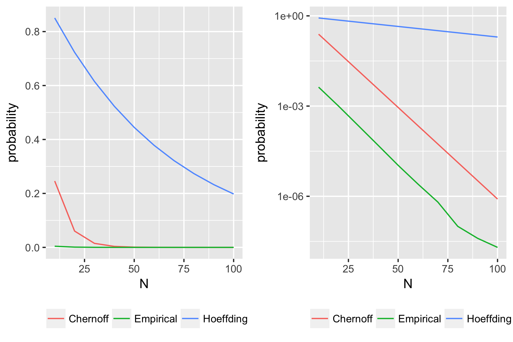
Now this is much better! By taking into account the means of $X_i$, we get a much tighter bound when those means are very small.

Final Notes

The primary reference for these notes is Prof. Roman Vershynin’s High Dimensional Probability, which I highly recommend. I also found these notes by Prof. John Duchi to be helpful. Also many thanks to Prof. Stefan Steinerberger and Prof. John Lafferty whose classes got me first interested in the topic.

These notes focused on sums of Bernoulli variables, but the field of concentration inequalities is remarkably deep. For example, please see Vershynin’s book for extensions of these inequalities for sub-Gaussian and sub-Exponential variables, which I did not write about here. Also, please contact me (Twitter or Email) for comments or questions!